GraphGym Tutorial and Neural Architecture Search
Robert Dyro, Ricky Grannis-Vu
Managing Experiments with GraphGym
By Ricky Grannis-Vu and Robert Dyro as part of the Stanford CS224W course project.
Graphs can be used to model a variety of objects and their relations, such as social network profiles and their connections or proteins and their interactions. Within a graph, these objects are represented by nodes, and their relations are represented by edges, where an edge between two nodes indicates that they are related.
Graphs can be used within many applications, such as predicting whether two social network profiles should be matched based on similar interests, or recommending a product to a user based on their prior product purchases. For many such problems, graph neural networks (GNNs) are used to learn meaningful representations (knows as embeddings) of nodes and/or edges in the problem's graph which we can use for downstream tasks, such as node classification or link prediction. However, designing a GNN to solve a given problem can be very difficult. There are thousands of possible GNN models, and finding the best GNN designs out of the GNN design space for different tasks can differ drastically [1].
GraphGym [1] lets us easily explore the GNN design space for a problem. Users can quickly set up GNN designs and experiment configurations and then explore thousands of different GNN designs in parallel. Furthermore, these experiment details are completely contained within configuration files, allowing users to easily share experiments for reproducibility and educational purposes. The GraphGym platform was originally developed by You et al. (2020) in their paper "Design Space for Graph Neural Networks" [1], and it has since risen in popularity and become integrated with PyTorch Geometric (PyG) [2].
In this tutorial, we will explore how we can use GraphGym to design a GNN to classify academic papers by high-level topic. We depict a high-level visualization of the GraphGym workflow below; in this tutorial, we will provide a detailed walkthrough of each step in the workflow below.
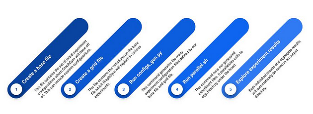
Figure 1: High-level GraphGym workflow
The Task
In our approach, we use the "Cora" sub-graph dataset within the larger CitationFull dataset [3]. Within the "Cora" dataset, academic papers are represented by nodes and a citation between two academic papers is represented by an edge between the two corresponding nodes. In addition, academic papers have associated meta-information which is represented by various node features. Each academic paper can be best described by a single-high level topic, which we refer to as its classification. In total, the "Cora" dataset contains 19,793 nodes; 126,842 edges; 8,170 node features; and 70 classes.
Our task is to determine what high-level topic best represents each academic paper, or node, within our graph datasets. Thus, our task can be modeled as a node classification problem.
We will design a GNN which, when trained, will be able to accurately classify each node in our graph datasets. We will hold out 20% of our data for evaluation. We will use a transductive training approach, meaning that we will use the full dataset during training but mask out many of the labels and predict different splits of these labels during training and evaluation.
Setting Up and Running a Single Experiment
Let's get started by setting up GraphGym. To do so, we need to clone the
GraphGym GitHub repository, enter the GraphGym/ directory, and install necessary dependencies.
$ pip install torch torch-scatter torch-sparse torch-cluster torch-spline-conv torch-geometric
$ git clone https://github.com/snap-stanford/GraphGym
$ cd GraphGym
$ pip install -r requirements.txt
We can use GraphGym to run experiments that explore the GNN design
space, helping us find the best GNN architecture for a given problem. To
set up an experiment, we need to create a *.yaml file that describes the experiment configuration. Let's create a new
file named paper_classification.yaml.
$ touch paper_classification.yaml
Next, open up the newly-created paper_classification.yaml file in your preferred editor. First, let's add the
following line:
out_dir: results
This line specifies that GraphGym should output the results of the
experiments to a directory named results once
the experiments finish.
Next, on to our experiment configurations. There are four high-level
things we need to configure to run an experiment: our dataset
configuration, our training configuration, our model architecture
configuration, and our optimizer configuration. We'll walk through how
we set up each of these configurations within our
paper_classification.yaml experiment
configuration file. First, let's start with our dataset configuration.
Add the following lines to describe our dataset configuration:
dataset:
  format: PyG
  name: Cora
  task: node
  task_type: classification
  transductive: true
  split: [0.8, 0.2]
  transform: none
Here, we specify that the dataset is in PyG format and that the dataset to use is Cora. We then specify that the dataset's task is node classification. We divide our data into an 80/20 train/test split, and we specify that our task is transductive. GraphGym further allows transforms to be applied to your dataset prior to training; however, for this task we will not apply any transforms to our dataset.
The next step is to add our training configuration. Add the following lines to the configuration file:
train:
  batch_size: 32
  eval_period: 20
  ckpt_period: 100
This specifies that a batch size of 32 should be used during training, and that evaluation should be performed every 20 epochs, with a checkpoint of our model weights saved every 100 epochs.
Our model architecture design and configuration is up next --- add the following lines to the configuration file:
model:
  type: gnn
  loss_fun: cross_entropy
  edge_decoding: dot
  graph_pooling: add
gnn:
  layers_pre_mp: 1
  layers_mp: 2
  layers_post_mp: 1
  dim_inner: 256
  layer_type: generalconv
  stage_type: stack
  batchnorm: true
  act: prelu
  dropout: 0.0
  agg: add
These lines let GraphGym know to use a GNN architecture with four
layers: two for message passing, and one each for before and after
message passing. Each layer is a convolutional layer, stacked on top of
each other, with sum aggregation. The GNN architecture has a hidden size
(dim_inner) of 256. Batch normalization and
PReLU activation function layers are used. Note that Dropout layers can
be used in GraphGym; however, for this model we do not use any Dropout.
The model uses a dot product operation to obtain edge embeddings. Since our problem is a classification problem, we calculate the model's loss using a cross-entropy loss function.
Finally, add the following lines to our configuration file to configure our optimizer:
optim:
  optimizer: adam
  base_lr: 0.01
  max_epoch: 400
Here, we tell GraphGym to use an Adam optimizer with a base learning rate of 0.01. We further tell GraphGym to train our model for up to 400 epochs.
Putting it all together, our complete experiment configuration file looks like:
out_dir: results
dataset:
  format: PyG
  name: Cora
  task: node
  task_type: classification
  transductive: true
  split: [0.8, 0.2]
  transform: none
train:
  batch_size: 32
  eval_period: 20
  ckpt_period: 100
model:
  type: gnn
  loss_wqfun: cross_entropy
  edge_decoding: dot
  graph_pooling: add
gnn:
  layers_pre_mp: 1
  layers_mp: 2
  layers_post_mp: 1
  dim_inner: 256
  layer_type: generalconv
  stage_type: stack
  batchnorm: true
  act: prelu
  dropout: 0.0
  agg: add
optim:
  optimizer: adam
  base_lr: 0.01
  max_epoch: 400
💡 If you are interested in exploring additional and more advanced experiment configuration options, or if you are interested in learning what the default values for the configuration options are, you can find the full list of experiment configuration options and their default values here.
Now that we have finished setting up the paper_classification.yaml experiment configuration file, we are all set to run
the experiment! To run the experiment, run the below line in your shell.
(As a reminder, you should still be in the GraphGym/ directory.)
$ python3 run/main.py --cfg paper_classification.yaml --repeat 3
This runs GraphGym with our experiment configuration
(--cfg paper_classification.yaml). To make our
experiment resilient to randomness, GraphGym allows us to optionally run
our experiment multiple times, with different random seeds. We can
specify how many times we would like to run our experiment with the
optional command-line flag: --repeat [num_times_to_run]. Here, we run our experiment three times, each time with a
different random seed, by adding —-repeat 3.
Once GraphGym finishes running our experiment, the experiment results
will be automatically saved in a directory named
results/paper_classification/. (Remember that
we specified within our paper_classification.yaml configuration file that our experiment results should be saved in an
output directory named results.)
When you enter this directory, you should see a few different
subdirectories. Since we ran our experiment three times, you should see
three numbered subdirectories (e.g.
results/paper_classification/2/), with each
subdirectory containing the experiment results for a run on a different
random seed. You should also see a subdirectory
results/paper_classification/agg/. This
subdirectory contains the experiment results aggregated over all the
random seeds.
Running a Batch of Experiments
So far we've been able to use GraphGym to run a single experiment. This allows us to easily test our chosen set of configurations and evaluate the performance of this combination of model architecture, training, optimization, and dataset options. But to get the best-performing model, we need to find the configuration options that lead to the best experiment performance. To do this, we must repeatedly vary our experiment configurations and see whether the changes improve or reduce our model's performance.
This can take a while! And doing this by hand is particularly time-consuming. Fortunately, GraphGym allows us to quickly test thousands of different configuration options in parallel, enabling us to easily find the best designs.
The first step is to create a base file for your experiments. This is
the set of initial configuration options which GraphGym will modify to
explore different experiment configurations. We can use the
paper_classification.yaml file we created in
the previous section as our base file.
The next step is to create a grid file. This file lists the
configuration modifications which GraphGym will explore. Within the
file, we provide a list of possible values which we would like to try
out for each of the configuration options which we would like to
experiment with. To get started, let's create a new file within the
GraphGym/ directory named grid.txt.
$ touch grid.txt
Next, open up the newly-created grid.txt file
in your editor of choice. Add the following lines to grid.txt:
train.batch_size batch_size [8,16,32,64,128]
gnn.dim_inner dim_inner [32,64,128,256,512]
gnn.act activation ["relu","prelu","elu"]
Each line specifies a different configuration option which we would like
to experiment with. Here, we specify that we would like to test
modifications to three configuration options: the training batch size,
the hidden size (dim_inner) of the GNN, and
the activation function used in the GNN.
Each line contains three values, separated by spaces. The first value on
the left is the name of the configuration option which we would like to
vary. This should be the same name as in your base file
(paper_classification.yaml).
The second value in the middle is an alias for the name of the configuration option --- it's a more readable version of the official name of the configuration option which GraphGym will use to refer to the configuration option. You can alias each configuration option anything you like.
The third value on the right is the list of values to try out for that configuration option. Here, we specify lists of different numbers to try out for the batch size and GNN hidden size, and a list of different activation functions to try out for the GNN activation function.
💡 There is one important formatting rule when writing your grid.txt file --- make sure your file contains no spaces except for the spaces separating each of the three values.
Using GraphGym, we can generate a bunch of experiment configuration
files from our base file and grid file. Each configuration file will
specify the configuration options for one experiment, where each
experiment is a modification of your base experiment according to the
modifications specified by your grid file. To generate your experiment
configuration files, make sure you are in the GraphGym/ directory and run the following command in your shell:
$ python3 run/configs_gen.py --config paper_classification.yaml --grid grid.txt --out_dir configs
This generates the many experiment configuration files from our base
file (paper_classification.yaml) and our grid
file (grid.txt) and stores them in a
subdirectory named configs/.
Now that we have generated all of our experiment configuration files, we are all set to run our experiments! GraphGym allows us to easily run all of our experiments and parallelize our experiment runs. To run the experiments, run the following command in your shell:
$ bash run/parallel.sh configs/paper_classification_grid_grid 3 10
Let's unpack this command. This command runs experiments for each of our
many generated experiment configuration files
(configs/paper_classification_grid_grid). Each
experiment is run 3 times, and 10 experiment runs are conducted in parallel at a time (if
you have a single GPU this last number should most likely be 1).
Once GraphGym finishes running our many experiments, the experiment
results will be automatically saved in a directory named
results/paper_classification_grid_grid/.
Within this directory, you should see a subdirectory for each of your
individual experiment runs (for each random seed). You should also see a
subdirectory results/paper_classification_grid_grid/agg/. This subdirectory contains the experiment results for each
of your differently configured experiments aggregated over all the
random seeds.
💡 For more information about the scripts used in this section, please see the Appendix at the end of this blog post.
Creating and Using Custom GraphGym Modules
As you have seen so far, GraphGym is a very powerful and useful framework! Using GraphGym, we can easily explore GNN designs in parallel from a range of configuration options in order to find the best GNN design for our task. But what if we would like to use a configuration option which GraphGym doesn't support? Maybe we have an idea for a new activation function or a new model architecture --- what do we do then?
Thankfully, GraphGym is a very flexible framework! One big highlight of GraphGym is that it allows users to easily register custom modules. Let's explore how we can create custom modules for our paper classification task.
To start, in our current grid file, we explore three activation functions: "relu", "prelu" and "elu". But what if we want to use a new activation function which GraphGym doesn't support? Let's try adding a new activation function: "tanh".
To do so, we need to create a file containing the code for our new
activation function. GraphGym will automatically support any new modules
which we add to the graphgym/contrib/
directory. Within the graphgym/contrib/
directory, you should see multiple subdirectories, such as act/, layer/, and
optimizer/. Each subdirectory corresponds to a
different type of module which we can create custom modules for. For
example, custom activation functions should be stored in the
graphgym/contrib/act/ directory.
Go ahead and create a new tanh.py file to
store our custom tanh activation function:
$ touch graphgym/contrib/act/tanh.py
Using your editor of choice, add the following lines to tanh.py to create a custom tanh activation function:
import torch
from graphgym.config import cfg
from graphgym.register import register_act

register_act('tanh', torch.nn.Tanh())
And that's it! We're ready to use our custom tanh activation function.
Since we named our activation function "tanh" in register_act(), to specify our activation function, you should
refer to it as "tanh" in our configuration files. For example, to
explore the addition of our tanh activation function within our
experiment batch, we can modify the corresponding line in grid.txt to include our "tanh" activation function:
gnn.act activation ["relu","prelu","elu","tanh"]
Now when you run an experiment batch to find the best performing GNN for classifying academic papers, your experiments will try using the "tanh" function as well. Pretty neat!
Advanced: Neural Architecture Search Example
💡 For our more advanced readers, in this section we provide an example of a larger custom creation to illustrate the power of GraphGym. You are welcome to skip this section if you are more interested in the high-level approach to GraphGym, but we highly recommend reading it to get an idea of how larger custom modules can be created with GraphGym.
In this more advanced section, we will walk through an example of how to create larger custom modules with GraphGym. We will create a Neural Architecture Search (NAS) model and, in the process, create a custom config and a custom GNN model within GraphGym. If you would like to view the complete code, feel free to explore this notebook.
Neural Architecture Search (NAS) is an automated process of designing neural network architectures, which can perform a specific task with high accuracy. NAS algorithms work by searching through a vast space of possible neural network architectures to find the best performing one. Typically, this process is guided by a reinforcement learning algorithm or a genetic algorithm, which evaluates the performance of each candidate architecture on a given task and then selects the best performing ones for further exploration. Random NAS is pretty much as good as genetic or reinforcement learning algorithms in practice, and GraphGym supports random NAS. We can use GraphGym to easily explore the search space of candidate architectures.
To do so, we need to create two custom GraphGym modules: a custom config and a custom GNN model. At a high level, we will use GraphGym to generate a batch of experiments, where each experiment corresponds to a different model architecture. We will define the possible components of our model architecture in a custom config file. Our custom GNN model will connect the components of any given model architecture together and output the results. Then, when we use GraphGym to run the various experiments, different components will be tried within our custom GNN model, and the best-performing GNN model will be saved.
Let's get started by creating the custom config. A config defines a set
of configurations which GraphGym can use during experiments. For
example, in our paper classification experiments, we used a few
pre-defined configs such as dataset:,
model:, gnn:, and
optim:. In our custom config, we will define a
set of configurable GNN model components (nodes and activation
functions) which our NAS can experiment with.
As a reminder, within the graphgym/contrib/
directory, you should see multiple subdirectories, such as act/, layer/, and
optimizer/. Go ahead and create a new file
named nas_config.py within the
graphgym/config/ subdirectory.
$ touch graphgym/contrib/config/nas_config.py
Next, using your editor of choice, go ahead and add the following lines to the file to create our custom config.
from yacs.config import CfgNode as CN
from graphgym.register import register_config

def set_cfg_nas(cfg):
    cfg.nas = CN()
    cfg.nas.node0 = "GCN"
    cfg.nas.node1 = "GCN"
    cfg.nas.node2 = "GCN"
    cfg.nas.node3 = "GCN"

    cfg.nas.node_0_1_act = "tanh"
    cfg.nas.node_0_2_act = "tanh"
    cfg.nas.node_0_3_act = "tanh"
    cfg.nas.node_1_2_act = "tanh"
    cfg.nas.node_1_3_act = "tanh"
    cfg.nas.node_2_3_act = "tanh"

register_config("nas", set_cfg_nas)
Since we named our config "nas" in register_config(), within our experiment configuration file, you should refer to
our config as nas:. Within the config, we
define individual configurations such as node0, node1, and node_1_3_act and initialize default values for each of them (in case the
configuration is not explicitly defined within our experiment
configuration file).
Once we have created our custom config, we can use it in our experiment configuration files! To use our custom config, you can specify it as follows within your experiment configuration file:
...
# nas config
nas:
  node_0_1_act: tanh
  node_0_2_act: tanh
  node_0_3_act: tanh
  node_1_2_act: tanh
  node_1_3_act: tanh
  node_2_3_act: tanh
  node0: GCN
  node1: GCN
  node2: GCN
  node3: GCN
...
And our custom config is ready to go!
💡 Fun fact: Creating custom/contrib configs had a bug in it previously. One of our team members, Robert, noticed and resolved the bug within the GraphGym GitHub repository: https://github.com/snap-stanford/GraphGym/pull/54.
The next step is to create our custom GNN model. As a reminder, our custom GNN model will connect together the components specified in our experiment configuration file and output the results.
We will store our custom GNN model in the
graphgym/contrib/network/ directory. Go ahead
and create a new file within this directory named nasgnn.py.
$ touch graphgym/contrib/network/nasgnn.py
And we add the following lines in nasgnn.py to
define our custom NAS GNN model architecture.
import torch
...
from graphgym.config import cfg
from graphgym.models.act import act_dict as inbuilt_act_dict
from graphgym.register import register_network
from graphgym.register import act_dict
...
act_dict = dict(act_dict, **inbuilt_act_dict, identity=lambda x: x)


class NASGNN(torch.nn.Module):
    def __init__(self, dim_in, dim_out, dropout=0.0, block_num=4):
        super().__init__()
    ...

    def forward(self, batch):
        x, edge_index, x_batch = batch.node_feature, batch.edge_index, batch.batch
    ...

register_network("nasgnn", NASGNN)
Since the main point which we wish to illustrate is how to define a custom GNN model architecture within GraphGym, we have removed the inner workings of the NAS GNN model architecture from the code cell above for the sake of readability. However, if you are interested in reading through the code for the NAS GNN model architecture, or are curious to copy over the code and try out the architecture yourself, please see our Appendix at the end of this blog post or access our complete notebook code here.
Since we named our model "nasgnn" in register_network(), within our experiment configuration file, you can specify
that you would like to use our custom "nasgnn" model by setting the
following configuration:
model:
  type: nasgnn
And there we have it! Our custom config and custom GNN model are ready to go. Let's go ahead and run an experiment using our custom modules. As before, we start by defining an experiment configuration file. You can copy over the experiment configuration file from Part 1 of this tutorial, and add the following lines to initialize our custom NAS model component configurations:
...
# nas config
nas:
  node_0_1_act: tanh
  node_0_2_act: tanh
  node_0_3_act: tanh
  node_1_2_act: tanh
  node_1_3_act: tanh
  node_2_3_act: tanh
  node0: GCN
  node1: GCN
  node2: GCN
  node3: GCN
...
And, as before, we next need to define a grid file to specify which values we should explore for our individual configurations within different experiments. For simplicity, let's suppose that we only wish to vary our custom model component configurations. We might define the following grid file:
nas.node_0_1_act node_0_1_act ["relu","prelu","tanh","identity"]
nas.node_0_2_act node_0_2_act ["relu","prelu","tanh","identity"]
nas.node_0_3_act node_0_3_act ["relu","prelu","tanh","identity"]
nas.node_1_2_act node_1_2_act ["relu","prelu","tanh","identity"]
nas.node_1_3_act node_1_3_act ["relu","prelu","tanh","identity"]
nas.node_2_3_act node_2_3_act ["relu","prelu","tanh","identity"]
nas.node0 node0 ["GCN","GAT","GraphSage","Identity"]
nas.node1 node1 ["GCN","GAT","GraphSage","Identity"]
nas.node2 node2 ["GCN","GAT","GraphSage","Identity"]
nas.node3 node3 ["GCN","GAT","GraphSage","Identity"]
Within this grid file, we specify that GraphGym should try out four different activation functions for each of our six activation configurations and four different GNN nodes for each of our four node configurations.
However, here we run into a small issue! By default, when we run GraphGym on a batch of experiments, it will try out every combination of possible values as defined in our grid file. However, in this case, the number of combinations this grid defines is:

This will take forever to explore with GraphGym!
Not all hope is lost however. When we run GraphGym on a batch of experiments, we can set an optional command-line flag which specifies that GraphGym should only run on a random sample of combinations defined in our grid file. This allows us to randomly subsample our configuration space and approach the optimal set of configurations in significantly less time. For example, to specify that GraphGym should sample 200 random combinations of configurations, add the following command-line flag when generating experiment configuration files in batch:
--sample --sample_num 200
Using this command-line flag, as you might recall from Section 2 of this blog post, the complete line which you can run in your shell to generate 200 experiment configuration files with random combinations of configurations is as follows:
$ python run/configs_gen.py --config configs/nas.yaml --grid configs/nas_grid.txt \
  --sample --sample_num 200
And then, as in Section 2 of this blog post, you can run our
newly-created batch of experiments by running the following line in your
shell. (As a reminder, the 5 below refers to
how many times we run each individual experiment on different random
seeds, and the 10 below refers to how many
jobs we will run in parallel.)
$ bash run/parallel.sh configs/nas_grid_nas_grid 5 10
After running 200 samples in our search space and averaging the results, we select the best GNN model architecture based on the final validation accuracy --- we are trying to generate architectures that generalize well and do not overfit. This was the winning GNN architecture during our run (running 200 samples, 5 times each, took us about 3.5h on a consumer GPU).
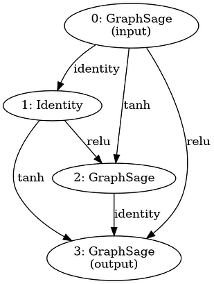
Figure 2: Diagram of winning GNN architecture during our run
Advanced: Monitoring GraphGym Experiments
💡 For our more advanced readers, in this section we walk through how to monitor GraphGym experiments using both TensorBoard and Ray. Monitoring neural network training is a critical step in ensuring that the model is learning correctly and making progress towards achieving its objective. During the training process, it's essential to monitor various metrics such as the loss function, accuracy, and validation metrics. By monitoring these metrics, we can adjust our hyperparameters, such as learning rate and batch size, to improve the performance of our model.
...with TensorBoard
Suppose that we return to our paper classification task and run our
batch of experiments. Depending on how many configuration combinations
we define, this might take a while! As our experiments are running, the
results will continuously aggregate in our results directory, which for
our paper classification task is
results/paper_classification_grid_grid.
We can monitor the progress of our experiments using TensorBoard. (If you're unfamiliar with TensorBoard, you can learn more about TensorBoard here. To set up TensorBoard to monitor our GraphGym experiments, after we start running our batch of experiments, run the following line in your shell:
$ tensorboard --logdir results/paper_classification_grid_grid
Then, all you have to do is navigate to http://localhost:6006/. There, you should see the TensorBoard dashboard displayed, allowing you to easily monitor the progress of your experiments. Pretty neat!
...with Ray
Ray is a great tool for parallelizing and monitoring hyperparameter tuning. Here, we demonstrate how to quickly set up Ray to parallelize and monitor GraphGym experiments. The first step is to set up Ray. We won't go into the details about how to set up Ray here, but if you are interested in learning more about Ray and how to set it up, please follow the instructions here. Assuming you have Ray set up on your local machine, let's dive into how we can run Ray for a batch of experiments.
Suppose that we have generated our set of experiment configuration files as usual. As a reminder, we can generate our set of experiment configuration files by running the following line in shell:
$ python run/configs_gen.py --config configs/classic.yaml --grid configs/classic_grid.txt
Now that our experiment configuration files are ready to go, let's start writing a script in Python to set up Ray to monitor our batch of experiments. As a reminder, we will not discuss the Ray code in depth as we assume some initial knowledge about Ray and how to set it up in Python. The first step is to create a new file to store our Python script and add the following lines of code:
classic_config = Path("").absolute() / "configs" / "classic.yaml"
classic_grid = Path("").absolute() / "configs" / "classic_grid.txt"
assert classic_config.exists()
assert classic_grid.exists()
print(gen_configs(classic_config, classic_grid))
config_dir = Path("").absolute() / "configs" / f"{classic_config.stem}_grid_{classic_grid.stem}"
assert config_dir.exists()
config_paths = list(glob(str(config_dir / "*.yaml")))
assert len(config_paths) > 0
So far, we have generated and discovered all of our experiment configuration files. Next, add the following lines of code:
def experiment_fn(config):
    # our custom config from the ray config
    config = config["custom_config"]
    repeats = config.get("repeats", 1)
    trial_name = config["trial_name"]
    grid_name = config["grid_name"]

    # write the config file passed by dict (since we want to allow distributed ray clusters)
    config_file_contents = config["config_file_contents"]
    config_file_contents.setdefault("dataset", dict())
    dataset_path = Path("/tmp/graphgym_datasets")
    dataset_path.mkdir(parents=True, exist_ok=True)
    config_file_contents["dataset"]["dir"] = str(dataset_path)
    config_path = Path("configs") / grid_name / f"{trial_name}.yaml"
    config_path.parent.mkdir(parents=True, exist_ok=True)
    config_path.write_text(yaml.dump(config_file_contents))

    # run the actual experiment
    run_config(config_path, repeats, verbose=config.get("verbose", True))

    # find the results
    result_path = (
        Path(re.sub(r"(^|/)configs/", r"\1results/", str(config_path.parent))) / trial_name
    )
    all_stats = dict()
    for key in ["train", "val", "test"]:
        stats_file = result_path / "agg" / key / "stats.json"
        print(f"Looking under {stats_file} for stats file")
        if stats_file.exists():
            all_stats[key] = read_graphgym_stats_file(stats_file)

    # finally, we'll return the final result
    return dict(all_stats)
We won't dive into the internals of the experiment_fn() function too closely. At a high-level, this function runs a
single experiment and outputs the results. It has three main parts.
First, experiment configuration files are reformatted as dictionaries
using YAML representation. This is necessary in order to run Ray on a
cluster. Second, we call the function run_config() to run our experiment using the reformatted configuration file.
Third, we extract the results from the resulting results files and
return the results as a dictionary.
The next step is to set up a set of Ray experiments, where each
experiment is set up to call our experiment_fn() function for an individual experiment configuration file. We can do
so with the following lines of code:
# we will convert config_paths into a list of configs with config read out using yaml
configs = [
    {
        "repeats": 1,
        "config_file_contents": yaml.safe_load(Path(config_path).read_text()),
        "trial_name": Path(config_path).stem,
        "grid_name": Path(config_path).parent.stem,
        "verbose": False,
    }
    for config_path in config_paths
]

# we'll only specify one field, custom_config because we're generating samples ourselves
ray_configs = {"custom_config": ray.tune.grid_search(configs)}

# by specifying resources, we're implicitly specifying how many jobs should run in parallel
resources_per_trial = {"cpu": 1, "gpu": 0.5}

# now, we define experiments using our ray function
experiments = ray.tune.Experiment(
    "graphgym_experiment",
    experiment_fn,
    config=ray_configs,
    resources_per_trial=resources_per_trial,
)
And, at long last, we have to run our experiments! Add the following line of code to run our experiments using Ray:
results = ray.tune.run_experiments(experiments=experiments)
Finally, let's collect the experiment results (which we collected in
experiment_fn()) and output the results as
they come in. We can do so with the following code:
for experiment in results:
    config = experiment.config
    print(config)
    print(f"Validation accuracy was {experiment.last_result['val'][-1]['accuracy']}")
    print("#######################")
Go ahead and run the complete Python script to run the batch of experiments using Ray. After you run the script, you can monitor the progress of the experiments in the Ray dashboard at localhost:8265.
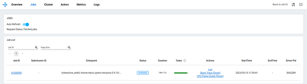
Figure 3: Screenshot of Ray dashboard
In Conclusion...
Many graph applications use GNNs to learn embeddings of nodes and/or edges, which can be used for downstream tasks, such as our paper classification problem. However, with thousands of possible GNN models to choose from, it can be a daunting task to design the right GNN architecture for the job as the best GNN design for different tasks can vary significantly.
As we have seen, GraphGym is a powerful tool that lets us easily explore the GNN design space for a problem. We have walked through how we can use GraphGym to explore thousands of different GNN designs in parallel. Furthermore, we have shown through example the flexibility of GraphGym to incorporate custom modules as necessary, ensuring that we can use GraphGym for various graph applications. GraphGym experiments can be integrated with many state-of-the-art machine learning infrastructure tools, such as monitoring tools TensorBoard and Ray. Overall, we hope we have demonstrated the power and flexibility of GraphGym, which make it an ideal choice for designing GNN models.
To see the complete code used in this tutorial blog post, please see our GitHub link here.
References
[1] You, J., Ying, R., & Leskovec, J. (2020) Design Space for Graph Neural Networks. NeurIPS. https://arxiv.org/abs/2011.08843
[2] Fey, M. & Lenssen, J. E. (2019) Fast Graph Representation Learning with PyTorch Geometric. arXiv. https://arxiv.org/abs/1903.02428
[3] Bojchevski, A. & Gunnemann, S. (2017) Deep Gaussian Embedding of Graphs: Unsupervised Inductive Learning via Ranking. arXiv. https://arxiv.org/abs/1707.03815
[4] Kingma, D. P. & Ba, J. (2014) Adam: A Method for Stochastic Optimization. arXiv. https://arxiv.org/abs/1412.6980
[5] Liu, H., Simonyan, K., & Yang, Y. (2018). Darts: Differentiable architecture search. arXiv preprint arXiv:1806.09055. Chicago
Appendix
A. GraphGym script details
1. GraphGym/run/main.py
usage: main.py [-h] --cfg CFG_FILE [--repeat REPEAT] [--mark_done] ...

GraphGym

positional arguments:
  opts             See graphgym/config.py for remaining options.

optional arguments:
  -h, --help       show this help message and exit
  --cfg CFG_FILE   The configuration file path.
  --repeat REPEAT  The number of repeated jobs.
  --mark_done      Mark yaml as done after a job has finished.
2. GraphGym/run/configs_gen.py
usage: configs_gen.py [-h] [--config CONFIG] --grid GRID [--sample]
                      [--sample_alias SAMPLE_ALIAS] [--sample_num SAMPLE_NUM]
                      [--out_dir OUT_DIR] [--config_budget CONFIG_BUDGET]

optional arguments:
  -h, --help            show this help message and exit
  --config CONFIG       the base configuration file used for edit
  --grid GRID           configuration file for grid search
  --sample              whether perform random sampling
  --sample_alias SAMPLE_ALIAS
                        configuration file for sample alias
  --sample_num SAMPLE_NUM
                        Number of random samples in the space
  --out_dir OUT_DIR     output directory for generated config files
  --config_budget CONFIG_BUDGET
                        the base configuration file used for matching
                        computation
3. GraphGym/run/agg_batch.py
usage: agg_batch.py [-h] --dir DIR [--metric METRIC]

Train a classification model

optional arguments:
  -h, --help       show this help message and exit
  --dir DIR        Dir for batch of results
  --metric METRIC  metric to select best epoch
B. Custom Model Code for Neural Architecture Search Example
Detailed NAS implementation
Here, we show how we design the custom NAS Graph Neural Network. We implement a custom NAS class by:
- generating our network blocks and activation functions from the configuration files
- implementing a custom forward function
Custom NAS Network
First, we define the blocks in our network
def __init__(self, dim_in, dim_out):
  ...
  block_num = block_num if "block_num" not in cfg.nas else cfg.nas.block_num
  self.blocks = nn.ModuleList()
  for i in range(block_num):
      self.blocks.append(self.build_conv_model(cfg.nas[f"node{i}"])(dim_in, dim_in))
  self.activations = nn.ModuleDict()
  for i in range(block_num):
      for j in range(i + 1, block_num):
          self.activations[f"{i}_{j}"] = deepcopy(act_dict[cfg.nas[f"node_{i}_{j}_act"]])
  self.post_mp = GNNNodeHead(dim_in=dim_in, dim_out=dim_out)
  ...
For activations, we have activations from all previous blocks to all subsequent ones.
Next, we can implement the forward function:
def forward(self, batch):
  x, edge_index, x_batch = batch.node_feature, batch.edge_index, batch.batch
  ...
  block_inputs = [[x]] + [[] for _ in range(1, len(self.blocks))]
  latest_output = x
  for i, block in enumerate(self.blocks):
      # apply the block to all its inputs and sum the output
      block_output = sum(
          F.dropout(block(x, edge_index), p=self.dropout, training=self.training)
          for x in block_inputs[i]
      )
      # record the latest output (for output)
      latest_output = block_output
      for j in range(i + 1, len(self.blocks)):
          # apply the specified activations to the output of the block for other blocks
          block_inputs[j].append(self.activations[f"{i}_{j}"](block_output))
  x = latest_output
  ...
Within the forward function, we iterate over cells and pass the outputs of all previous cells through them.
C. Validation Accuracy vs. Iteration Time for Neural Architecture Search Example
In our Neural Architecture Search example, we can also plot the validation accuracy vs iteration time which lets us quantify the tradeoff between latency and performance of the network. Interestingly higher latency networks are more expensive to evaluate but do not achieve better performance --- the trend peaks around 0.022 seconds per iteration.
We plot the validation accuracy and iteration time for a classic hyperparameter search of the inner dimension of a graph convolution network (GCN) --- the simple case.
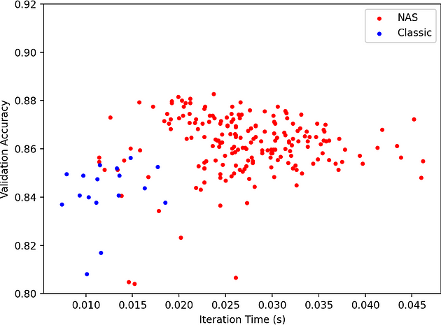
Figure 4: Graph plotting validation accuracy vs. iteration time
We also show the validation accuracy vs epoch during training for a random sample within our NAS search space and the best architecture. The best architecture does not overfit!
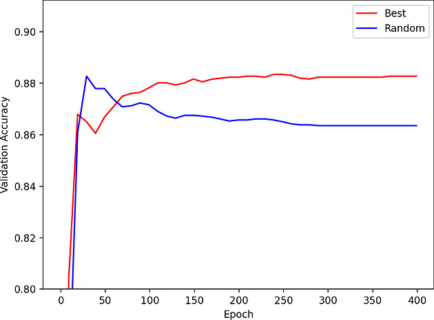
Figure 5: Graph plotting validation accuracy vs. epoch for a random sample within the NAS search space and the best architecture