Post-training Compression of Neural Network via SVD
Robert Dyro
|
|
|
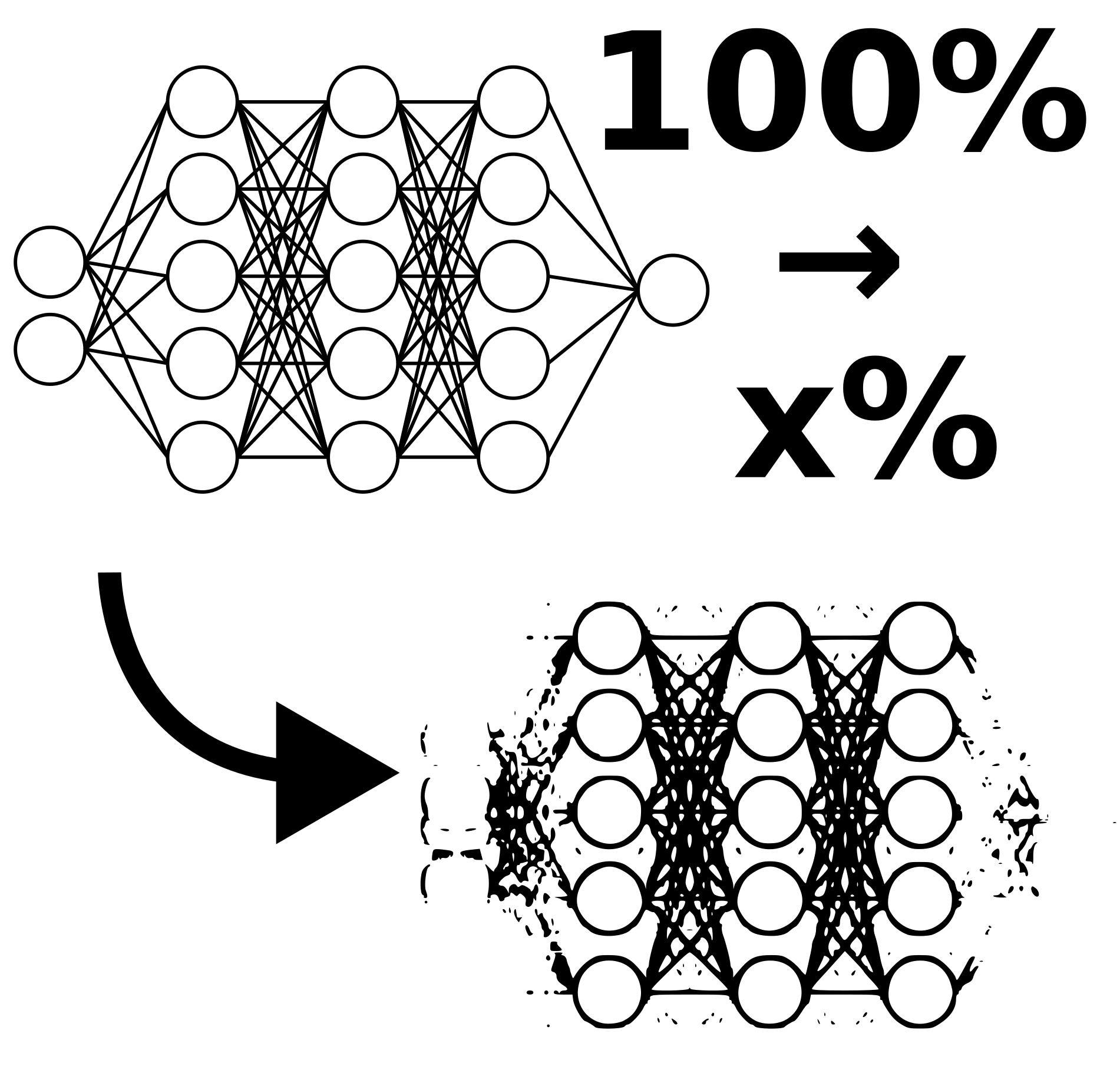
Fig: Approximating trained NN weights using SVD. |

Introduction
A well known demonstration of how singular value decomposition (SVD) can extract the most important features of a matrix is image compression where only a couple of components from the full SVD decomposition of the original image are retained. When the image is reconstructed, it tends to resemble the original one, but the representation occupies much less space. The compression ratio can often result in a 100x reduction in size (compared to a naive storage).1
Here's an algorithm for compressing an image using SVD:
- Read the image into a matrix (if the image has many channels, execute this algorithm for every channel)
- decompose the image matrix to SVD components , where
- .
- .
- .
- .
- (you can use a truncated SVD to only compute the first components)
- means constructing a diagonal matrix from the input vector
- retain only the first components by whatever means of choosing (probably inspecting the reconstruction error)
- is the compressed image
- the compression ratio, how much less information we're storing to represent the image is just
- * or if we want to target a particular compression fraction
Compression Ratio === This approach is commonly known in literature as T-SVD (truncated SVD).
|
|
|
Fig: SVD image compression, retaining only 5 principal components, for a compression to 2% of original information. |
Question: Can we use SVD to compress a neural network?
The idea behind this project is to investigate whether an SVD compression can be used to reduce the memory (storage) footprint of a trained neural network (NN) after it has been trained.

Post-training Compression
This problem is addressed in the field of post-training compression of NNs. Most approaches to reducing the model footprint focus exclusively on only 1 type of target for compression: matrix weights. Biases, activations, buffers and other learned parameters are typically much smaller in size to weights and so are left uncompressed. Weights are typically:
- linear layer weight flatted convolutional layer weight where is the convolutional layer weight
- and is the flattened weight
linear projection layer in an attention layer The most popular post-training compression technique is quantization where the compression target matrices are converted from single- (float32) or half-precision (float16) floating point numbers into 4-bit or 8-bit integers. There are multiple ways to do this, the simplest of which is to just round to the nearest point on an equally space grid from the minimum to the maximum in the range.
where is the number of bits available.
Finally, the computation with quantized weights is typically done by dequantizing the matrix into the smallest floating point representation that does not introduce numerical problems, usually half-precision (float16) and performing regular matrix multiplication with the right hand-side.
For much faster matrix multiplication, the matrix is usually dequantized in small optimized blocks to make best use of the modern GPU architectures' local memory cache and fastest memory access patterns.
SVD Compression
The SVD compression of a matrix is an extremely simple technique. For every weight to compress, we compute and then retain only the first components, so that
Combining SVD and Quantization
Because quantization both results in enormous memory savings and can be applied to any matrix, we use quantized SVD compression as the technique of choice in this project.
where is not quantized, because its size is usually negligible.
Experimental Approach
We investigate the combined SVD + quantization compression technique on 4 different, representative and popular neural networks
- vision model VGG-19
- vision model ResNet-101
- NLP model BERT
- NLP model Phi-2
We use the excellent bitsandbytes library to perform the compression. We do
not propose to focus on the inference speed of this combined SVD + quantization
compression scheme; that would require writing custom GPU kernels which is
outside the scope of this work. Presumably, the smaller the model footprint, the
faster the inference speed as matrix-multiplication is often memory-bound.
Deciding on the compression fraction is a bit of an art. As a way to make the experiments tractable, we decide on the following rank selection rule:
set compression rank to a value that produces an error of less than on an batch example input
Since the error is a monotonic function of , we can use binary search to find the smallest that satisfies the error condition.
def evaluate_error(k: int) -> float:
    self.rescale(CompressionConfig(Compression.SIZE_K, k))
    with torch.no_grad():
        new_output = self.forward(input)
    err = torch.norm(new_output.to(output) - output) / torch.norm(output)
    return err
Finally, if the required error cannot be satisfied without exceeding such a that the compression ratio is > 1.0, we simply change the layer back to its linear form. No need to use SVD if we would exceed the number of parameters of the linear layer.
Results
VGG19 ImageNet Classification Model
We start with the VGG19 network trained on ImageNet. The inspiration for this starting point is in the Sparse low rank factorization for deep neural network compression paper.2
The reason why VGG model family is an attractive target for SVD weight compression is because over 90% of model parameters are contained in the extremely large linear classifier layers at the end of the network.
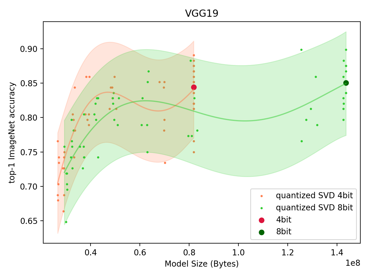
By scanning the layer error threshold , we create and plot two dependent variables: the model size (in bytes) vs a performance measure. For VGG19, performance is the top-1 accuracy on the ImageNet validation set.
For VGG19, we only compress the linear layers (in the classifier).
|
|
|
Fig: Performance of Quantized SVD VGG19 model. |
ResNet-101 ImageNet Classification Model
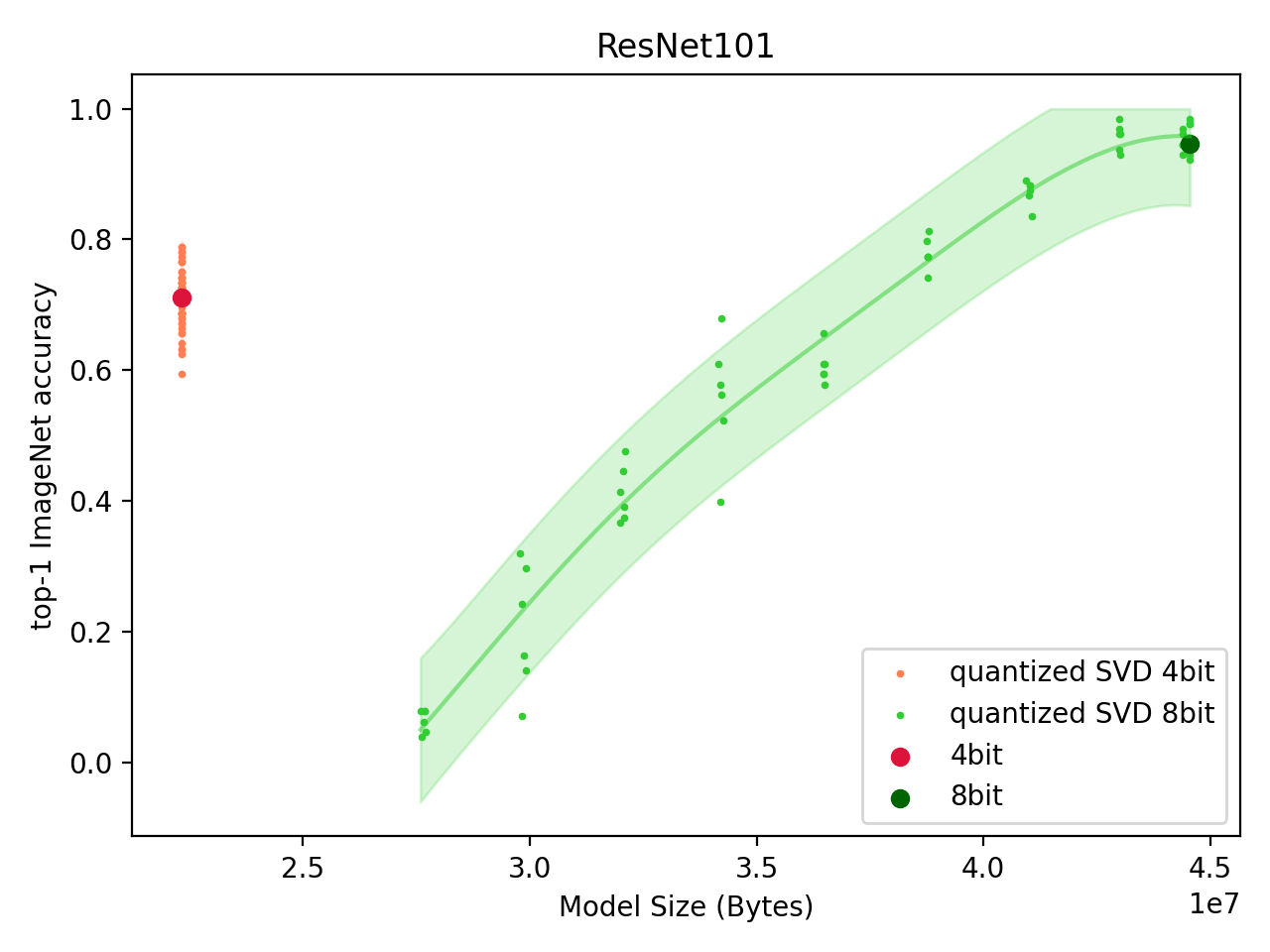
Following from VGG19, we turn to the ResNet-101 model. The ResNet model family contains linear layers, but they are much smaller. The vast majority of parameters is contained in the convolutional layers. We compress both the linear layers and the convolutional layers, the latter by first flattening all, but the first (output channels) dimension -- thus converting the 4D convolutional layer weight into a 2D matrix.
|
|
|
Fig: Performance of Quantized SVD ResNet-101 model. |
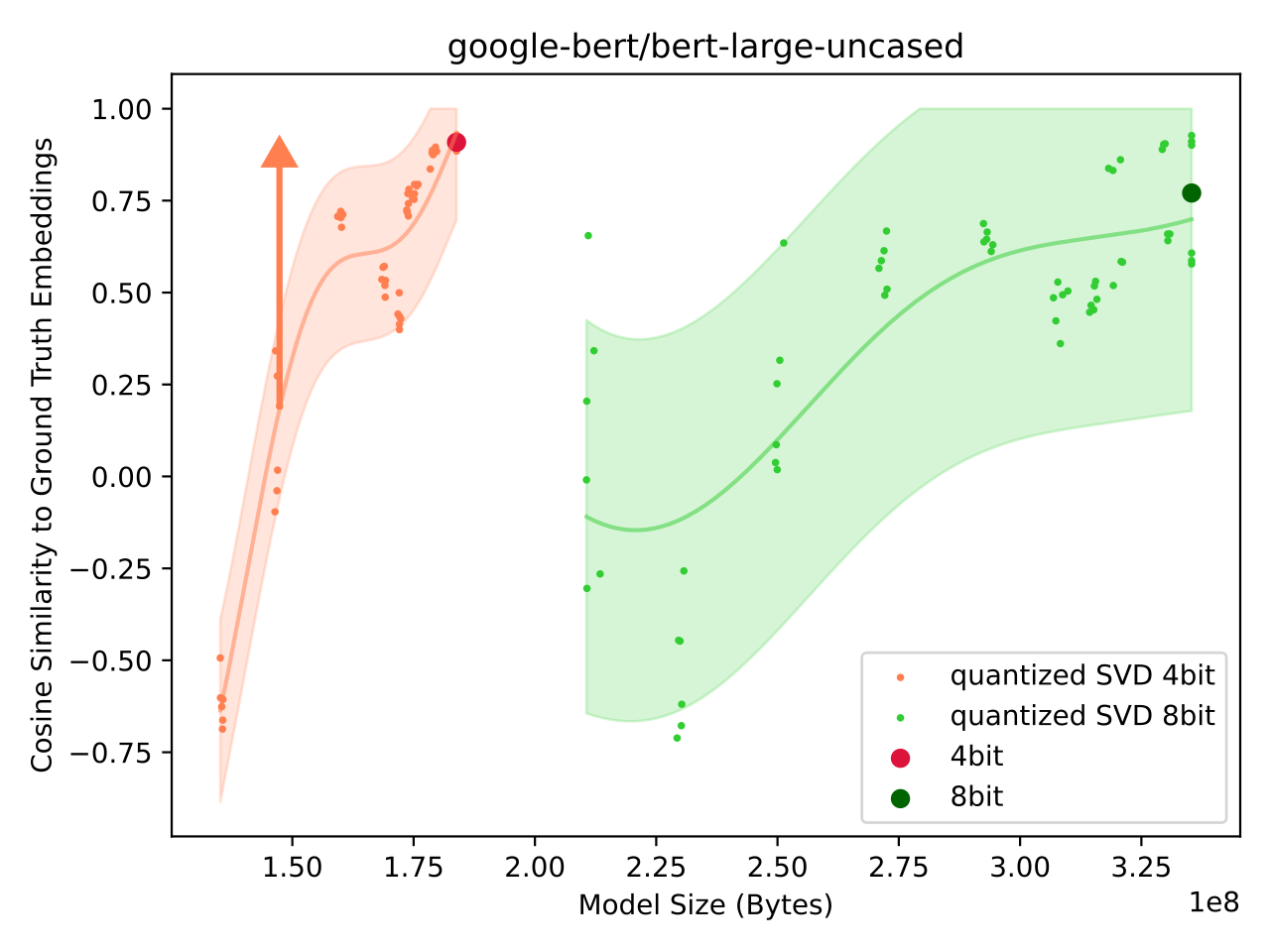
BERT
After ResNet, we attempt to compress the BERT model. BERT is a transformer model with the vast majority of components being the linear weight matrices used for the attention projections:
- key projection .
- query projection .
- value projection .
All of which are linear layers.
The BERT model is not a classifier, at least in its base form, so we compare the cosine similarity of the final pooler embeddings between an uncompressed (float32) and a compressed (SVD + quantization) model.
|
|
|
Fig: Performance of Quantized SVD BERT model. |
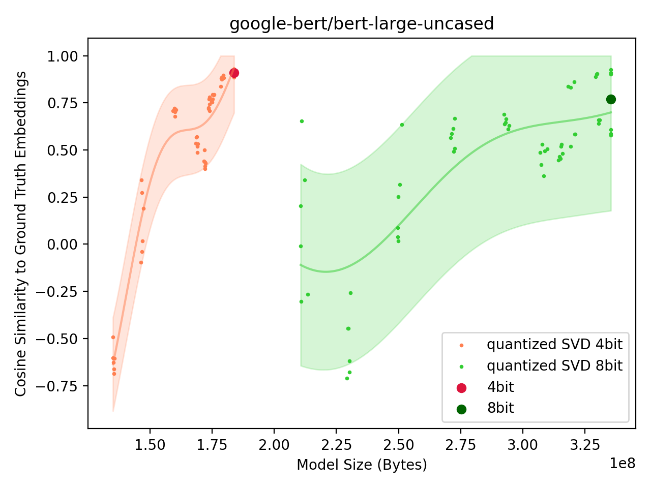
A cosine similarity of 1.0 means the two vectors are aligned, 0.0 means they are uncorrelated. The result of the model achieving a cosine similarity of -0.5 is odd as random vectors should have a cosine similarity of 0.0.
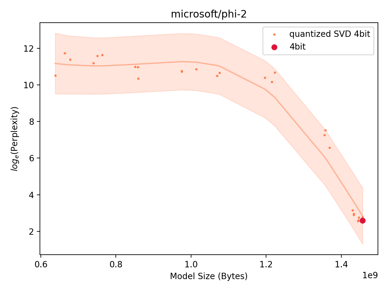
Phi-2
Finally, we take a look at a small LLM (SLM). The Phi-2 model is a 2.7B model for which the vast majority of parameters are contained in transformer layers, so linear layers (the attention projections). Here, the performance metric is the perplexity of the model on a validation set.
Low perplexity means the model predicts the ground-truth next word in a text well. It is defined as the exponentiation of the cross-entropy loss.
|
|
|
Fig: Performance of Quantized SVD Phi-2 model. |
Discussion and Conclusions
The truncated SVD does not appear to be a particularly useful compression method. It is also extremely noteworthy that quantization is a very effective way of scaling the model down.
Existing academic literature includes several competing compression ideas
- different rank selection rules - sometimes based on retraining
- while we could use another selection rule, the optimal rank selection is an NP in the number of layers since the error is not a monotonic function of -s when several layers are considered at the same time
- selection rules based on validation data risk overfitting to the validation data and losing model's generalization ability
another low-rank factorization of the weight matrix and model retraining to recover performance
this approach is much more principled, as observed in the literature (e.g., GPTQ: Accurate Post-Training Quantization for Generative Pre-trained Transformers), the actual optimization problem we need to consider when compressing a matrix is
where is the input data, thus is merely an approximation. Then again, using in the optimization problem risks overfitting to a validation set. Nevertheless, of course, we are guilty of this ourselves -- our binary rank search also uses example inputs.
Recovering Performance Through Brief Retraining
|
|
|
Fig: Performance of Quantized SVD BERT model. |
In the face of terrible results, we need to find another approach. What is particularly surprising about quantization is that despite being performed per-layer, with error introduced to each layer independently, it does not degrade global performance very much. This is in stark contrast to the truncated SVD approach investigated here. SVD is an optimal compression method under the operator norm, but it does not appear to be a particularly useful compression method for neural networks -- perhaps with the exception of VGG19 where the majority of parameters are contained in a single linear layer.
We should to abandon our initial assumption of not using data to fine-tune the model. The obvious next step involves looking at the network error globally. Instead of compressing every layer independently, we should compress the network as a whole. This leads to two possible ideas, investigated to some degree in the literature:
- compress the concatenated network parameter vector
- it is not immediately obvious how to apply SVD here, parameters being a vector and not having a clear matrix structure
- if we considered the weights as a block diagonal matrix and applied SVD there, this is mathematically equivalent to compressing each layer with SVD independently
- compress the network initially - producing a low-rank approximation to a
matrix weight, then briefly retrain the entire network to recover a better
global low-rank approximation for each layer
- while perhaps useless as a compression method, SVD decomposition could be a good initialization for a low-rank factorization of the weight matrix
Work in progress...
References
Work in progress...
@article{swaminathan2020sparse,
  title={Sparse low rank factorization for deep neural network compression},
  author={Swaminathan, Sridhar and Garg, Deepak and Kannan, Rajkumar and Andres, Frederic},
  journal={Neurocomputing},
  volume={398},
  pages={185--196},
  year={2020},
  publisher={Elsevier}
}
Some people point out that while the original image is often stored as bytes, the results from SVD decomposition are double precision numbers, which occupy 8x the space of a byte. In reality, SVD decomposition is computed in double (or single) precision numbers, but the result can be easily quantized to bytes without much loss of numerical accuracy since the vectors, the result of SVD, are orthonormal and thus, typically do not have a large numerical range.↩
Sparse low rank factorization for deep neural network compression↩